optuna.visualization.matplotlib.plot_edf
-
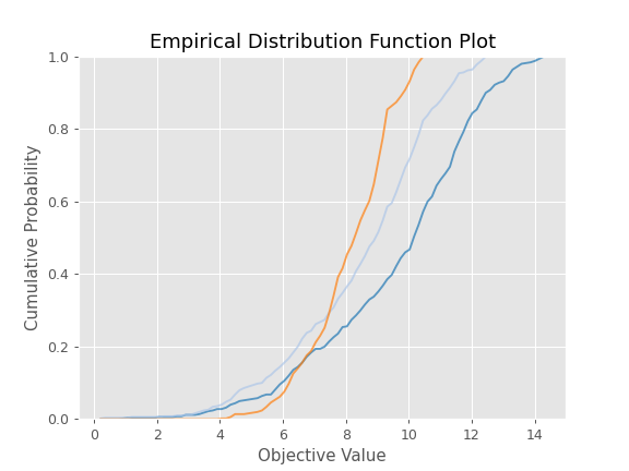
optuna.visualization.matplotlib.plot_edf(study: Union[optuna.study.Study, Sequence[optuna.study.Study]]) → matplotlib.axes._axes.Axes[source]¶ Plot the objective value EDF (empirical distribution function) of a study with Matplotlib.
See also
Please refer to
optuna.visualization.plot_edf()for an example, where this function can be replaced with it.Example
The following code snippet shows how to plot EDF.
import math

import optuna


def ackley(x, y):
    a = 20 * math.exp(-0.2 * math.sqrt(0.5 * (x ** 2 + y ** 2)))
    b = math.exp(0.5 * (math.cos(2 * math.pi * x) + math.cos(2 * math.pi * y)))
    return -a - b + math.e + 20


def objective(trial, low, high):
    x = trial.suggest_float("x", low, high)
    y = trial.suggest_float("y", low, high)
    return ackley(x, y)


sampler = optuna.samplers.RandomSampler(seed=10)

# Widest search space.
study0 = optuna.create_study(study_name="x=[0,5), y=[0,5)", sampler=sampler)
study0.optimize(lambda t: objective(t, 0, 5), n_trials=500)

# Narrower search space.
study1 = optuna.create_study(study_name="x=[0,4), y=[0,4)", sampler=sampler)
study1.optimize(lambda t: objective(t, 0, 4), n_trials=500)

# Narrowest search space but it doesn't include the global optimum point.
study2 = optuna.create_study(study_name="x=[1,3), y=[1,3)", sampler=sampler)
study2.optimize(lambda t: objective(t, 1, 3), n_trials=500)

optuna.visualization.matplotlib.plot_edf([study0, study1, study2])
- Parameters
study – A target
Studyobject. You can pass multiple studies if you want to compare those EDFs.- Returns
A
matplotlib.axes.Axesobject.
Note
Added in v2.2.0 as an experimental feature. The interface may change in newer versions without prior notice. See https://github.com/optuna/optuna/releases/tag/v2.2.0.